HDR

This command is used to construct an HDR bearing element object in three-dimension. The 3D continuum geometry of an high damping rubber bearing is modeled as a 2-node, 12 DOF discrete element. This is the third element in the series of elements developed for analysis of base-isolated structures under extreme loading (others being ElastomericX and LeadRubberX). The major difference between HDR element with ElastomericX is the hysteresis model in shear. The HDR element uses a model proposed by Grant et al. (2004) to capture the shear behavior of a high damping rubber bearing. The time-dependent values of mechanical properties (e.g., vertical stiffness, buckling load capacity) can also be recorded using the "parameters" recorder.

For a 3D problem:

element HDR $eleTag $Nd1 $Nd2 $Gr $Kbulk $D1 $D2 $ts $tr $n $a1 $a2 $a3 $b1 $b2 $b3 $c1 $c2 $c3 $c4 <<$x1 $x2 $x3> $y1 $y2 $y3> <$kc> <$PhiM> <$ac> <$sDratio> <$m> <$tc>

---

$eleTag	unique element object tag
$Nd1 $Nd2	end nodes
$Gr	shear modulus of elastomeric bearing
$Kbulk	bulk modulus of rubber
$D1	internal diameter
$D2	outer diameter (excluding cover thickness)
$ts	single steel shim layer thickness
$tr	single rubber layer thickness
$n	number of rubber layers
$a1 $a2 $a3 $b1 $b2 $b3 $c1 $c2 $c3 $c4	parameters of the Grant model
$x1 $x2 $x3	vector components in global coordinates defining local x-axis (optional)
$y1 $y2 $y3	vector components in global coordinates defining local y-axis (optional)
$kc	cavitation parameter (optional, default = 10.0)
$PhiM	damage parameter (optional, default = 0.5)
$ac	strength reduction parameter (optional, default = 1.0)
$sDratio	shear distance from iNode as a fraction of the element length (optional, default = 0.5)
$m	element mass (optional, default = 0.0)
$tc	cover thickness (optional, default = 0.0)

Physical Model and Mechanical Properties

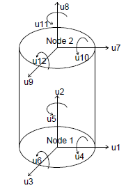
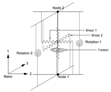
The physical model is considered as a two-node, twelve degrees-of-freedom discrete element. The two nodes are connected by six springs that represent the mechanical behavior in the six basic directions of a bearing. The degrees of freedom and discrete spring representation of an elastomeric bearing is shown in the below figures.

The general form of element force vector, <math>{{f}_{b}}</math>, and element stiffness matrix,<math>{{K}_{b}}</math> , for element representation considered above is given by equation below:

<math>{{f}_{b}}=\left[ \begin{matrix}

  Axial  \\
  Shear1  \\
  Shear2  \\
  Torsion  \\
  Rotation1  \\
  Rotation2  \\

\end{matrix} \right];\ \ \ \ \ \ {{K}_{b}}=\left[ \begin{matrix}

  Axial & 0 & 0 & 0 & 0 & 0  \\
  0 & Shear1 & Shear12 & 0 & 0 & 0  \\
  0 & Shear21 & Shear2 & 0 & 0 & 0  \\
  0 & 0 & 0 & Torsion & 0 & 0  \\
  0 & 0 & 0 & 0 & Rotation1 & 0  \\
  0 & 0 & 0 & 0 & 0 & Rotation2  \\

\end{matrix} \right]</math>

The coupling of the two shear springs is considered directly by using a coupled bidirectional model. All other springs are uncoupled. The coupling of vertical and horizontal directions are considered indirectly by using expressions for mechanical properties in one direction that are dependent on the response parameters in the other direction. Linear uncoupled springs are considered in the torsion and the two rotational springs as they are not expected to significantly affect the response of an elastomeric bearing. The off-diagonal terms due to coupling between axial and shear, and axial and rotation, are not considered in the two-spring model (Koh and Kelly, 1987) used here. An exact model would have non-zero values of these off-diagonal terms. A discussion on the formulation of the two-spring model and the exact model is presented in Ryan et al.(1991). The subscript b refers to the element’s basic coordinate system. Response quantities are transformed between the basic, local and global coordinates to perform computations.

The discrete spring model presented here has the advantages of easy implementation and being computationally efficient. The mechanical properties of the six springs (also referred to as material models in OpenSees) are defined using analytical solutions available from the analysis of elastomeric bearings. The expression for mechanical properties, including stiffness and buckling load capacity, are derived using explicit consideration for geometric nonlinearity due to large displacement effects. The P-Delta effect, which is an approximate method to account for geometric nonlinearity in structural analysis problems, is therefore not considered. The material models in six directions are:

• Axial direction: a new mathematical model that captures the behavior under cyclic tension Link
• Two shear directions: a bidirectional model proposed by Grant et al. (2004)
• Torsion: a linear elastic model
• Two rotational directions: linear elastic models

In addition to the behavior captured by existing bearing elements, this element can capture the following:

1. Degradation of bearing stiffness and damping due to scragging effects in shear
2. Cavitation and post-cavitation behavior in tension
3. Variation in critical buckling load capacity due to lateral displacement
4. Variation in vertical axial stiffness with horizontal displacement

Recorders

In addition to regular recorders provided by the bearing elements ( Element Recorder), this element can also record instantaneous values of cavitation force (Fcn), buckling load capacity (Fcrn), and vertical stiffness (Kv) using the "Parameters" recorder in that order.

        Example: recorder Element <-file $fileName> -time <-ele ($ele1 $ele2 ...)> Parameters
        recorder Element -file param.out -time -ele 1 Parameters

To check if bearing has buckled or cavitated, an user can obtain the histories of Fcn and Fcrn as described above and divide the axial force (obtained from basicForce recorder, qb(2)) by Fcn and Fcrn at each time step, which provides demand vs capacity (D/C) ratios at each time step. If Fcn/qb(0) > 1.0 : Cavitation, or Fcrn/qb(0)>1.0 : Buckling.

Examples

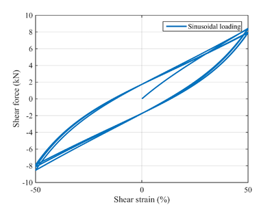
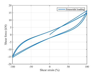
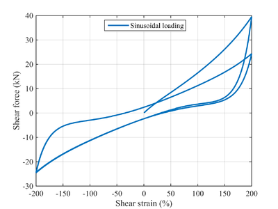
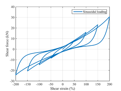
An example is presented here, in which a high damping rubber bearing (bearing KL301 in Grant et al. (2004)) is subjected to different amplitudes and sequences of loading. The bearing (KL301) and parameters of Grant's model presented in Grant et al. (2004) have been used. The tcl files can be found here: File:HDRgravity.tcl File:HDRtest.tcl

References

1. Kumar, M., Whittaker, A., and Constantinou, M. (2014). "An advanced numerical model of elastomeric seismic isolation bearings." Earthquake Engineering & Structural Dynamics, Published online, DOI: 10.1002/eqe.2431. Link
2. Grant, D. N., Fenves, G. L., and Whittaker, A. S. (2004). "Bidirectional modeling of high-damping rubber bearings." Journal of Earthquake Engineering, 8(sup001), 161-185.
3. Kumar, M., Whittaker, A., and Constantinou, M. (2015). "Experimental investigation of cavitation in elastomeric seismic isolation bearings." Engineering Structures, 101, 290-305. Link
4. Kumar, M., Whittaker, A., and Constantinou, M. (2015). "Response of base-isolated nuclear structures to extreme earthquake shaking." Nuclear Engineering and Design (In press). Link

---

Code Developed by: Manish Kumar, University at Buffalo, SUNY.

Any bugs in this element can be reported to mkumar2 AT buffalo dot edu