Site Response Analysis of a Layered Soil Column (Total Stress Analysis)
Example prepared by: Christopher McGann and Pedro Arduino, University of Washington
Return to OpenSees Examples Page
This article describes the OpenSees implementation of a site response analysis a soil deposit located above an elastic half-space using total stress analysis. A single soil column is modeled in two-dimensions and is subject to an earthquake ground motion in a manner which accounts for the finite rigidity of the underlying medium.
Provided with this article are three input files which execute this analysis in different ways.
- freeFieldSingle.tcl has a single soil layer for simplicity and is intended to outline the basic analysis approach.
- freeFieldIndepend.tcl and freeFieldDepend.tcl are two approaches to a comparison study with the 1D wave propagation analysis tools ProShake and ProShakeNL (http://www.proshake.com/). Each approach breaks the soil up into a series of sublayers, however, one uses the PressureIndependMultiYield material with user-generated modulus reduction (G/Gmax) curves while the other uses the PressureDependMultiYield material with automatically-generated G/Gmax curves.
Also included is the velocity time history of the selected ground motion, velocityHistory.out. This file is required for the analysis.
Several helpful files are included as well:
- GilroyNo1EW.out, the acceleration time history for the selected ground motion, as downloaded from the Peer NGA strong motion database, with the header information removed.
- processMotion.m, a Matlab script which reshapes the GilroyNo1EW.out acceleration history into a column vector, then integrates this using the trapezoidal method to obtain the velocity time history needed for the site response analysis.
- accelPlot.m and respSpectra.m, Matlab scripts which produce the verification plots included in this article from the recorded results.
Download them all in a compressed file: siteResponseAnalysis.zip
To run this example, the user must download the one of the input files and the velocity time history file, velocityHistory.out, and place them in a single directory. Once this has been done, the user can then run the analysis. The Matlab scripts and the acceleration time history files are not essential to the analysis, however, they are provided to demonstrate how an alternative acceleration time history can be converted into the analysis and how certain plots can be obtained from the recorded output.
A large set of similar examples has been developed at the University of California at San Diego. They are available at http://cyclic.ucsd.edu/opensees. These examples utilize a wide variety of element and material formulations, as well as different boundary and loading conditions than those used in this example. The user is referred to these examples for further information on how to set up a site response model in OpenSees.
Model Description
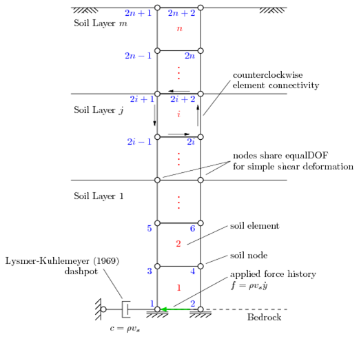
In this article, the site response analyses are performed for soil deposits which are underlain by an elastic half-space, which simulates the finite rigidity an underlying medium such as bedrock. It is assumed that there is no groundwater, therefore, total stress analysis is used in this example. The soil is modeled in two-dimensions with two degrees-of-freedom using the plane strain formulation of the quad element element. The provided input files consider only a single layer of soil, however, the files freeFieldIndepend.tcl and freeFieldDepend.tcl, consider a soil profile which has a parabolically-increasing shear wave velocity profile with depth. This is accomplished using sublayers, thus, the use of multiple soil layers in an OpenSees site response analysis is demonstrated. A general schematic of the model is shown in Fig. 1. In this example, the horizontal direction is the first degree-of-freedom and the vertical is the second. The soil node, element, and layer numbering schemes all begin at the bottom.
Note: The remainder of the main model description in this article, when not otherwise specified, refers to the simpler of the three provided input files, freeFieldSingle.tcl, with the intention of highlighting the main site response analysis details. The other input files are essentially the same, with the main difference being the complexity introduced by the inclusion of multiple layers. The more complex files are explained later in this article during the discussion of the comparison study.
To account for the finite rigidity of the underlying half-space, a Lysmer-Kuhlemeyer (1969) dashpot is incorporated at the base of the soil column using a zeroLength element and the viscous uniaxial material. The Lysmer-Kuhlemeyer (1969) dashpot is assigned a dashpot coefficient equal to the product of the mass density and shear wave velocity of the underlying layer with the area of the base of the soil column. In this example, the properties of a bedrock layer are used for the half-space. The soil column is excited at the base by a horizontal force time history which is proportional to the known velocity time history of the ground motion. Further information on this modeling approach can be found in Joyner and Chen (1975) and Lysmer (1978) among others.
The horizontal force time history is applied as a Path TimeSeries object using the file, velocityHistory.out. The force history is obtained by multiplying the known velocity time history by a constant factor set as the product of the area of the base of the soil column (width x thickness) with the mass density and shear wave velocity of the underlying layer. The area of the soil column is included to ensure proportional loading for any desired horizontal element size. The provided Matlab script, processMotion.m, shows how the velocity time history was obtained from the selected acceleration time history.
Soil Profile Geometry
For the simple soil profile considered in the file freeFieldSingle.tcl, the soil profile geometry is controlled entirely by the thickness of the soil deposit. In this example, this value is set at 40 meters.
In the multi-layered soil profiles in the other input files, the soil profile geometry is controlled by a specified number of layers and the thicknesses of each individual soil layer. In this case the overall thickness of the soil profile is the sum of the layer thicknesses.
Mesh Geometry
The geometry of the mesh is based upon the concept of resolving the propagation of the shear waves at or below a particular frequency by ensuring that an adequate number of elements fit within the wavelength of the chosen shear wave. This ensures that the mesh is refined enough such that the desired aspects of the propagating waves are well captured in the analysis.
This is accomplished in the model by specifying the highest frequency which the user wishes to be well resolved and the number of elements that the user desires to be in one wavelength of a shear wave propagating at this frequency. The wavelength used to define the mesh geometry is determined by dividing the minimum shear wave velocity of the soil profile by the specified cutoff frequency. In the provided examples there are either 8 or 10 elements per wavelength. The largest value possible value for the specified frequency is the sampling frequency of the ground motion. The provided examples use 100 Hz for the cutoff frequency.
The horizontal size of the elements is set to be the minimum vertical element size in the soil column. The number of nodes and the total number of elements are computed automatically. The number of elements is based on the computed element size and the thickness of the soil deposit. For n total elements, there are 2n + 1 total nodes.
Soil Nodes
The soil nodes are created automatically from the input geometry and meshing information. As shown in Fig. 1, the node numbering scheme is left-to-right, top-to-bottom. Nodes with even numbers fall on the y-axis, and the odd-numbered nodes are spaced horizontally by the computed horizontal element size.
Dashpot Nodes
A single zeroLength element is used to define the Lysmer-Kuhlemeyer (1969) dashpot, therefore, only two nodes are required. These nodes are arbitrarily assigned numbers 2000 and 2001. If the user has modified the meshing information such that there are more than 2000 nodes in the soil column, the dashpot node numbers will need to be changed.
Boundary Conditions and Equal Degrees-of-Freedom
The nodes at the base of the column are fixed against displacements in the y-direction in accordance with the assumption that the soil layers are underlain by bedrock. The remaining soil nodes are then tied together using the equalDOF command in order to achieve a simple shear deformation pattern. This is done by declaring equalDOF for every pair of nodes which share the same y-coordinate.
One of the dashpot nodes is fully fixed (node 2000), while the other is fixed only against displacements in the y-direction (node 2001). To incorporate the dashpot element into the total model, equalDOF is again used, this time linking the horizontal degrees-of-freedom of the partially fixed dashpot node and one of the nodes at the base of the soil column.
Soil Material Properties and Objects
A series of material properties are required to define the constitutive behavior of the soil and the underlying elastic half-space. The main soil properties are the mass density, the shear wave velocity, and Poisson's ratio. From these, the elastic, shear, and bulk moduli are computed. Poisson's ratio is set as zero in these examples for the purposes of emulating a one-dimensional analysis. With Poisson's ratio at zero, no vertical accelerations are generated.
The remaining soil properties correspond to the particular constitutive model selected in each analysis, either PressureDependMultiYield or PressureIndependMultiYield. For these examples, these properties are largely based on the recommendations detailed on the PressureDependMultiYield or PressureIndependMultiYield pages of the OpenSees command manual.
For the case of multiple layers, one material object is created for each layer using the material properties defined in the input file. With the exception of a few global properties, each layer is given a separate set of properties.
During the creation of these examples is was noted that using too few yield surfaces in these nested surface models, or using poorly spaced user-generated surfaces, can cause high frequency shaking to develop in the model. This appears to be due to the way in which these constitutive models work. There is not one consistent tangent over the length of the backbone curve, instead, a smooth backbone curve is approximated using a series of linear segments. If there are too few, or poorly spaced, yield surfaces, a dramatic change in stiffness can occur as the stress path crosses a particular yield surface, resulting in a shock which is manifested as the observed high frequency shaking. This behavior can be alleviated by using a larger number of yield surfaces, resulting in a smoother approximation to the backbone curve of the soil. Care should be taken, however, depending upon the intentions of the analysis. As the number of surfaces increases, the time needed to complete the analysis also increases, and in the end, the inclusion of this high frequency shaking does not significantly alter the results of the simulation. It is recommended that the user keep these ideas in mind when selecting the number of surfaces to use in a particular analysis.
Soil Elements
Four-node quad elements are used to model the soil using the plane strain formulation of the quad element. The element connectivity uses a counterclockwise pattern for the previously-described node numbering scheme (see Fig. 1). The soil elements in each layer are assigned the material tag of the material object corresponding to that layer. A unit thickness is used in all examples. The self-weight of the soil is considered as a body force acting on each element. The body force is set as the unit weight of the soil in each layer, which is determined from the respective mass density input value.
Dashpot Material and Element
The viscous uniaxial material is used to define the Lysmer-Kuhlemeyer (1969) dashpot. This material model requires a single input, the dashpot coefficient, c. Following the method of Joyner and Chen (1975), the dashpot coefficient is defined as the product of the mass density and shear wave velocity of the underlying medium, which, in this example, is assumed to have the properties of bedrock. The dashpot coefficient must also include the area of the base of the soil column to maintain proportional results for any horizontal element size. Since the elements are created with unit thickness, this area is simply the computed horizontal element size.
A zeroLength element is used for the Lysmer-Kuhlemeyer (1969) dashpot. This element connects the two previously-defined dashpot nodes and is assigned the material tag of the Viscous uniaxial material object in the first degree-of-freedom (horizontal direction).
Recorders
The recorders defined for this example document the following items:
- the nodal displacements, velocities, and accelerations in both degrees-of-freedom
- the stress and strain response at each Gauss point in each element
The recorded nodal values are the true values for each parameter, not relative values as with the uniformExcitation command.
Two sets of recorders are included to capture the response of the soil during the gravity analysis (which is sometimes useful to ensure proper model generation) and the response of the soil during the application of the ground motion. These files are differentiated by a naming scheme in which the records corresponding to the gravity analysis are named 'Gacceleration', 'Gstress', etc ...
Gravity Loading and Analysis
The gravity analysis in this example is conducted as a transient analysis with very large time steps, thus simulating a static analysis while avoiding the conflicts which may occur when mixing static and transient analyses. The self-weight of the soil elements provides the loads, therefore, no loading object is required. Gravity is applied for ten steps with entirely elastic constitutive behavior. This allows the material objects to update various parameters to account for confining pressure. Once these steps have converged, the material objects are updated using the updateMaterialStage command to consider elastoplastic behavior, and the gravity analysis is repeated for 40 steps.
Horizontal Loading and Analysis
Using the method of Joyner and Chen (1975), dynamic excitation is applied as a force time history to the base of the soil column, at the node which shares equal degrees-of-freedom with the Lysmer-Kuhlemeyer (1969) dashpot. This force history is obtained by multiplying the velocity time history of the recorded ground motion by the mass density and shear wave velocity of the underlying bedrock layer and the area of the base of the soil column (the horizontal element size in these examples). This technique considers the finite rigidity of the underlying layer by allowing energy to be radiated back into the underlying material.
The force history is applied to the model as a Path TimeSeries object using a Plain load pattern object. The actual force applied to the node in each time step is the product of the load factor indicated in the pattern object (1.0 in this example), the additional load factor included in the timeSeries object, and the value found in the file, velocityHistory.out, at that time step. The load factor included in the timeSeries object is used to create a force history from the velocity history found in the namesake file.
The transient analysis is conducted with the Newmark integrator using the gamma and beta coefficients defined near the top of the input file. These values are set at 0.5 and 0.25, respectively to ensure there is no numerical damping in the analysis.
Since these models consider elastoplastic soil behavior, there is inherent hysteretic damping which occurs, however, a small amount of Rayleigh damping is used so there is still some damping at low strain values. The level of Rayleigh damping is controlled by the damping ratio and the circular frequencies of two modes of vibration. This type of approach is discussed in most dynamic analysis texts, such as Chopra (2007).
The time step used in the analysis is selected to meet stability considerations using the Courant-Friedrich-Lewy (CFL) condition (discussed well by LeVeque, 2007). Meeting the requirements of this condition ensures that the time step is small enough for stability given the maximum shear wave velocity and the minimum vertical element size in the model. The example files are set up such that the analysis time step and the corresponding number of steps are automatically generated to satisfy this condition. If the required time step is larger than the time step increment found in the recorded ground motion, the value specified in the ground motion is used. If the user alters the shear wave velocity profile such that the lowest layer does not have the highest shear wave velocity, then the value of $vsMax used in this routine will need to be updated.
Representative Results
Several plots displaying results obtained from running the example site response analysis from the file, freeFieldSingle.tcl, are provided for use as a means of verification. These plots were generated using the Matlab scripts accelPlot.m, and respSpectra.m, which are available for download with the rest of the files in a compressed folder here.
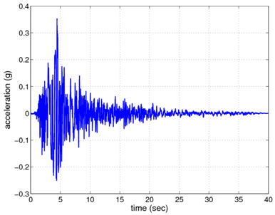
Fig. 2 shows the acceleration response at the ground surface (top of the soil column). This figure was created by simply plotting the recorded response at each time increment. The m-file, accelPlot.m was used to create the figure.
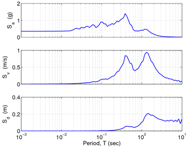
Fig. 3 shows the computed acceleration, velocity, and displacement response spectra at the ground surface. The figure was created using the m-files, accelPlot.m and respSpectra.m.
Comparison of Results with One-Dimensional Analysis Tools
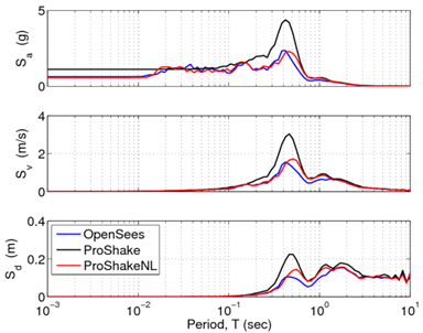
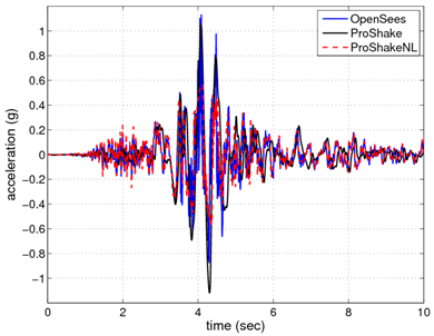
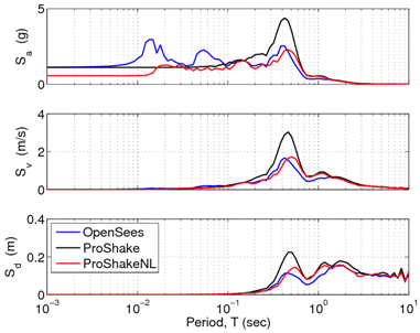
To validate the site response analysis framework used in these examples, a comparison study was accomplished using the one-dimensional, equivalent linear site response analysis program ProShake and the one-dimensional, nonlinear site response analysis program ProShakeNL. The input files freeFieldIndepend.tcl and freeFieldDepend.tcl were used for this purpose.
In the comparison study, a sand deposit having a parabolically-increasing shear wave velocity profile with depth was selected. This profile is implemented in OpenSees using 30 material layers, each having a specified shear wave velocity, which is then used to compute appropriate values for the shear and bulk moduli. It is important to note that the pressure dependency exponent is set to zero so the input values of shear and bulk modulus for each layer are not updated based on the overburden stress in each element.
The layering scheme was set up to match that used in the 1D analyses, with each layer having appropriate material parameters, and all analyses used the same ground motion applied to the base of the soil deposit. The 1D analyses include an infinite elastic half-space below the soil deposit, and these layers were assigned properties corresponding the bedrock properties used in the OpenSees analyses.
The two example input files represent two separate approaches to this comparison study. In the file, freeFieldIndepend.tcl, the soil is defined using the PressureIndependMultiYield nDMaterial, and the user-generated modulus reduction (G/Gmax) option is used, with the selected G/Gmax curves matching those used in the Shake analyses. Using this approach, the strength of each soil layer is defined entirely by the input G/Gmax data and the shear modulus value assigned to that layer. Parameters such as friction angle and cohesion are not used for this purpose. Though the material is called 'pressure independent', it is important to note that pressure dependency was manually introduced into the model by specifying the shear wave velocity of each layer. If it is also assumed that the confining pressure will not dramatically change during the excitation, then this approach becomes even more acceptable, especially in a free-field analysis where 2D elements are used to mimic a 1D analysis.
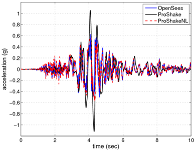
Figs. 4 and 5 show the surface acceleration histories and the response spectra at the surface, respectively, obtained from the analysis using the file, freeFieldIndepend.tcl, alongside the results obtained from ProShake and ProShakeNL. As shown, the OpenSees analysis correlates well with the results obtained using the nonlinear 1D analysis (ProShakeNL). It is interesting to note the differences between the equivalent-linear approach of ProShake and the nonlinear approaches used by OpenSees and ProShakeNL. As shown in Fig. 4, during the low amplitude shaking near the beginning of the motion, the ProShake results are significantly different from the others. In the nonlinear analyses, during this initial low amplitude shaking the response is elastic. Plastic behavior does not occur until the stronger shaking which occurs later in the motion. In the equivalent-linear approach, this type of response cannot be captured for a strong motion such as that used in this example. If the largest shaking is enough to produce plastic response, then the soil acts as if it is plastic during the entire motion. One way to use an equivalent-linear analysis tool to check nonlinear results is to use motions in which the amplitudes are scaled down.
The second comparison example, found in the file, freeFieldDepend.tcl, represents a more typical approach to a site response analysis of a sand profile in OpenSees. The PressureDependMultiYield nDMaterial is used, with soil properties corresponding to those used in the two Shake analyses, and automatically-generated yield surfaces (G/Gmax) curves. In this case, the constitutive model used the specified friction angle to define the strength of each layer, however, in order to maintain a shear wave velocity profile which corresponds to the other analyses, the pressure dependency exponent is set to zero and the shear wave values are input manually for each layer. If this was not a desired aspect of the analysis, a single material could be used along with a non-zero pressure dependency exponent to produce a pressure-dependent stiffness profile.
Figs. 6 and 7 show the surface acceleration histories and the response spectra at the surface, respectively, obtained from the analysis using the file, freeFieldDepend.tcl, alongside the results obtained from ProShake and ProShakeNL. As shown, the OpenSees analysis correlates well with the results obtained using ProShakeNL during lower amplitude shaking, though it deviates during the stronger shaking portions of the motion. The peak ground acceleration returned using this approach correlates fairly well with the equivalent-linear results, though this may be coincidental to the amount of Rayleigh damping used in the analysis.
This comparison study has demonstrated that a site response analysis conducted in OpenSees using the approaches detailed in these examples is capable of producing results which correlate well with commonly used site response analysis approaches. The approach that is selected should depend upon the objectives of the particular analysis in which they will be used. If the goal of the analysis is to emulate results obtained using a 1D analysis tool, the approach used in freeFieldIndepend.tcl is recommended, however, it is noted that care should be taken when attempting to use this approach in a two-dimensional analysis (i.e. more than just a single soil column). For 2D analyses, it is often easier and more realistic to define materials with pressure dependent strength, such as sands, using and approach similar to that in freeFieldDepend.tcl.
References
- Chopra, A.K. (2007). Dynamics of Structures, Third Edition, Pearson Prentice Hall.
- Joyner, W.B. and Chen, A.T.F. (1975). "Calculation of nonlinear ground response in earthquakes," Bulletin of the Seismological Society of America, Vol. 65, No. 5, pp. 1315-1336, October 1975.
- LeVeque, R.J. (2007). Finite Difference Methods for Ordinary and Partial Differential Equations, Society for Industrial and Applied Mathematics, Philadelphia.
- Lysmer, J. (1978). "Analytical procedures in soil dynamics," Report No. UCB/EERC-78/29, University of California at Berkeley, Earthquake Engineering Research Center, Richmond, CA.
- Lysmer, J. and Kuhlemeyer, A.M. (1969). "Finite dynamic model for infinite media," Journal of the Engineering Mechanics Division, ASCE, 95, 859-877.