Earthquake in Any Direction
Example posted by: Seyed Mohammad Javad Foroughi Moghadam (SMJ.Foroughi), International Institute of Earthquake Engineering and Seismology (IIEES)
In this example we want to apply earthquake in any direction to a 3D elastic frame by using UniformExcitation command in OpenSEES software.
All of the page can be download as a pdf file here:
- The main PDF file: File:Any direction earthquake.pdf
The main tcl file of the example can be download here:
- The main TCL file: File:AnyDirectionEarthquake.tcl
Apply Earthquake in Any Direction
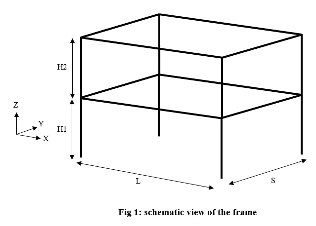
In this example we want to apply earthquake in any direction to a 3D elastic frame by using UniformExcitation command in OpenSEES software. Presented method is usable for any other 3D structure. In OpenSEES by UniformExcitation command we can apply acceleration in global directions. But it is not possible to apply acceleration in a direction other than global directions. To gain this end we have to rotate model through an introduced angle. So model geometry is dependent on that angle. The intended frame is a one bay two story elastic frame as in fig 1.
In this frame we tried to introduce parameters for all of geometric components. Parameters L and S are used for bay length in parallel with global X and Y directions, respectively (not rotated frame). H1 and H2 are story heights.
Model Dimension:
As it is a 3D frame model it has 3 dimension with 6 degrees of freedom at each node. So the model basic command is as follow: wipe ; model BasicBuilder -ndm 3 -ndf 6 ; Define Parameters: Parameters of this model are as follow:
- Define Parameters
set L 7.0 ; set S 4.0 ; set H1 3.0 ; set H2 3.0 ;
set Alpha 30.0 ; set Pi 3.14 ; set g 9.81 ;
- Loads (Kg/m2)
set DL 500.0 set LL 200.0 set ang [expr int($Alpha)] ; set FileName "OutPut_$ang" ; file mkdir $FileName ;
Parameters L, S, H1 and H2 are geometric parameters and defined with set command. Note that units that are used in this model are N, m and sec. Alpha is the angle between longitudinal direction of the frame and global X direction in degrees. DL and LL are distributed dead and live load of the floors in kg/m2. In last two lines we create a folder that contain the rotation angle in its name.
Define Nodes:
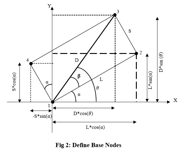
This step is one of the important steps in this model procedure as their coordinates have to define dependent to rotation angle. In fig 2 you can see location of base nodes as function of rotation angle. Other nodes of first and second floor are defined such base nodes with different Z coordinates. Global X and Y directions are shown un fig 2. We define nodes 1 to 4 as function of rotation angle, considering node 1 to be origin of the global coordinates. We define new parameter D to be diameter of the rectangular shape plan, also beta and theta are new angels that are shown in fig 2.
As angels have to define in radian we create new parameter, AlphaRad, to make degrees to radian for next calculations. All nodes of the frame are defined as follow:
Boundary Conditions:
In this frame all base nodes are fix to represent fix support as follow:
Define Elements:
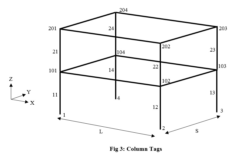
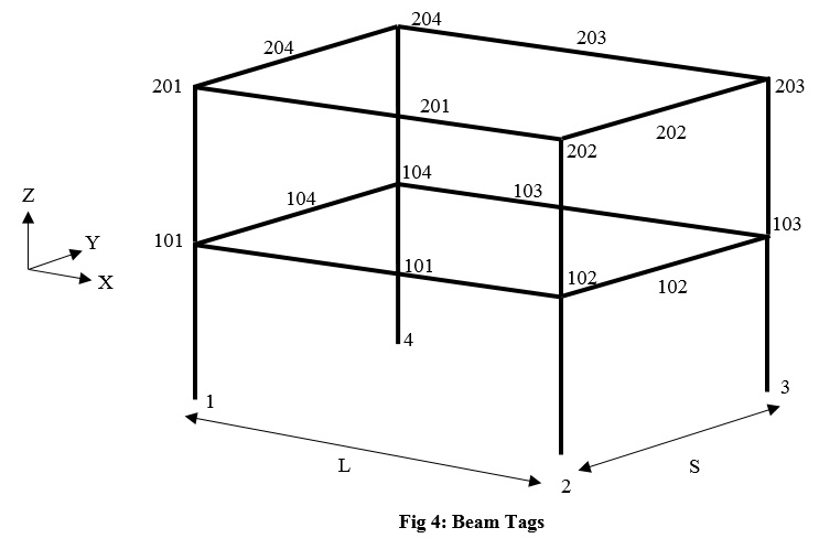
In this step we define elastic elements of the frame. The manner of numbering elements is shown in fig 3 and fig 4:
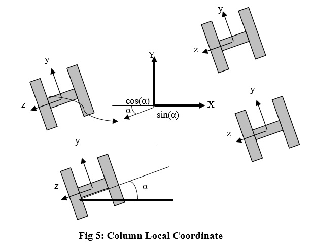
Before define elements we have to define geometric transformations of elements. We define a Linear transformation for beams and a PDelta transformation for columns. To calculate components of the geomTransf command pay attention to fig 5. Geometric transformations are defined as follow:
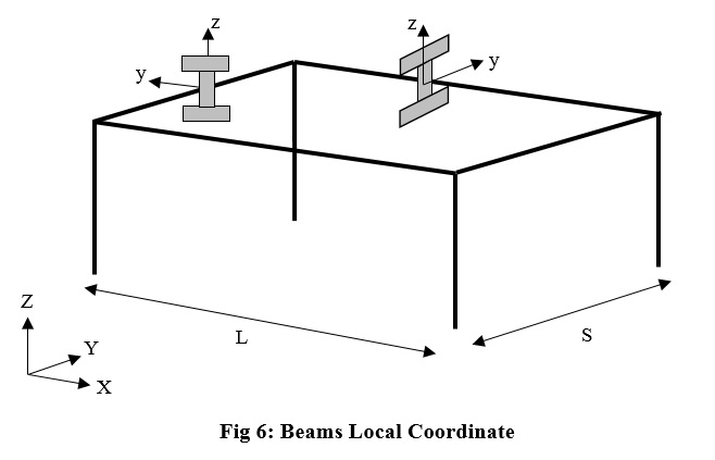
As it is shown from fig 5 geometric transformation of the columns is related to rotation angle. For beams we consider that the local weak axis is z, so to define transformation components, in all rotation angle local z axis is in the vertical (global Z) direction, and its transformation command is not related to the rotation angle. Fig 6 emphasis this point.
We use IPE270 for beams and IPB300 for columns. Now we can define elements of the model as follow:
For define column mass we consider a distributed mass, proportional to its section area. But for calculating beam mass, we consider mass of the floor and add it to elements mass.
Modal Analysis:
In this step we form an Eigen analysis to get principal frequency and period of the frame. As nature of the frame is unchanged by changing the rotation angle, it can use to test model geometry. In next lines we calculate Eigen values of the model:
Gravity Loading:
In this step we define distributed gravity loads on beams.
Static Analysis:
After defining gravity loads we have to perform a static analysis to apply gravitational loads to the model. This analysis procedure is as follow:
To ensure that static analysis have been performed successfully we set a sentence to appear after analysis by puts command.
Define Recorders:
Now we define required recorders as follow:
Seismic Loading:
In this step we define an acceleration to apply through a transient analysis to the model.
Acceleration file with name accel.txt is next to the model and we make it to a time series. Then by UniformExitation command we define direction of the earthquake to be global X direction. You see we define X direction, but as Alpha changes at the beginning of the model, direction of the earthquake will change.
Time History Analysis:
Now we perform a transient analysis to apply seismic load to the frame.
In the above commands parameter NInput is number of acceleration points in the accel.txt file, ndt is a number to divide steps to reduce length of analysis steps, dtAnalysis is the analysis time step and NAnalysis is the number of analysis steps.
RUN OpenSEES:
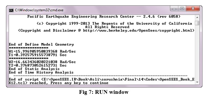
Now modeling is finished and we can RUN the model. After RUN model a window is opened as follow:
Results:
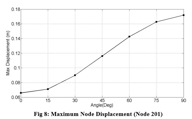
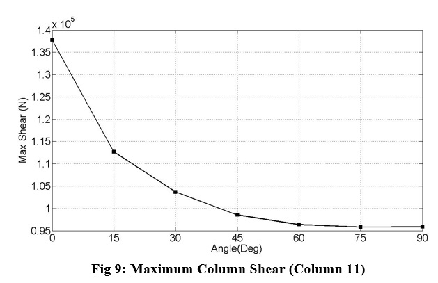
We change model direction from 0.0 to 90.0 degrees and compare results, such as max node displacement and max column shear between this rotation angles. Fig 8 and 9 presents this results:
As you can see maximum displacement increased by increase of rotation angle. In case of 90 degrees, seismic load applies to the weak direction of the frame and its max displacement is the largest displacement through other cases. In case of 0.0 degree, seismic load acts on strength direction of the frame and its maximum displacement is the minimum value through other cases.
Fig 9 compare column shear between rotation angle cases from 0.0 to 90.0 degrees. As it is shown maximum shear of the column decrease by increase of rotation angle.
References
- SMJ.Foroughi (2017). “The Most Complete Applied Reference of OpenSEES” Book (In Persian), [ http://www.opensees.ir/]
