One-dimensional Consolidation
Example prepared by: Christopher McGann and Pedro Arduino, University of Washington
This article describes the OpenSees implementation of a 1D consolidation model. A single soil column is modeled in two-dimensions, but all compression is one-dimensional. The model can consider either single or double drainage of the soil layer.
The input file needed to execute this analysis, 1Dconsolidation.tcl, is provided along with several helpful Matlab scripts to plot the results, plotPorePressure.m and plotStress.m.
Download them all in a compressed file: consolidation.zip
To run this example, the user must download the file 1Dconsolidation.tcl. Once this has been done, the user can then type "source 1Dconsolidation.tcl" into the interpreter of the OpenSees.exe application to run the analysis. The Matlab scripts are not essential to the analysis, however, they are provided to demonstrate how certain plots can be obtained from the recorded output.
Model Description
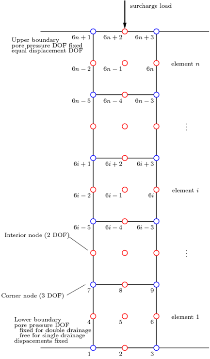
The one-dimensional consolidation model consists of a column of 9-node quadrilateral elements. These elements have two sets of nodes; the corner nodes have 3 degrees-of-freedom (2 displacement, 1 pore pressure), and the interior nodes have 2 displacement degrees-of-freedom only. These elements do not display the locking behavior associated with 4-node quadrilateral elements with pore pressure degrees-of-freedom, though the connectivity becomes more complex. A schematic depicting the 1D consolidation model is provided in Fig. 1. In this diagram, the corner nodes are blue and the interior nodes are red.
This example is able to consider both single and double drainage conditions for the soil layer. The user can specify the desired drainage condition using the variable drainage. Setting drainage to 1 gives single drainage, with zero pore pressure at the top of the soil layer. Setting drainage to 2 gives double drainage, with zero pore pressure at the top and bottom of the soil layer.
Mesh Geometry
The geometry of the finite element mesh used for this example is dependent on several parameters which must be specified by the user. These include the number and size of the elements in the horizontal direction (default values are 1.0) and the number and size of the elements in the vertical direction. In this example, there are 10 elements in the vertical direction, and the elements are square.
Corner Nodes
The corner nodes of the elements (depicted in blue in Fig. 1) are created in two dimensions, with three degrees-of-freedom (DOF). The first two DOF are displacements in the horizontal and vertical directions. The third DOF is for pore pressure. The input file provided with this example automatically generates the corner nodes in the proper locations depending on the parameters defined in the mesh geometry section.
All of the corner nodes are fixed against horizontal translation (first DOF). The nodes on the lower boundary are fixed against both horizontal and vertical translations.
The corner nodes at the upper boundary of the soil layer are fixed in the pore pressure DOF for the single and double drainage cases, while the corner nodes at the lower boundary are only fixed in the pore pressure DOF for the double drainage case.
Interior Nodes
The interior nodes of the elements (depicted in red in Fig. 1) are created in two dimensions, with two DOF. The input file provided with this example automatically generates these nodes in the proper locations based on the specified parameters in the mesh geometry section.
The single interior node at the lower boundary is fixed against horizontal and vertical translation. The interior nodes on the edges of the soil column are fixed against horizontal displacements.
The nodes on the upper boundary of the soil layer (both corner and interior) are given equal displacement DOF using the equalDOF command.
Soil Material
The soil in this example is assumed to be cohesive, therefore the nDMaterial PressureIndependMultiYield is used for the soil constitutive model. The various required material parameters (shear modulus, bulk modulus, permeability, etc...) are defined for this constitutive model based upon the assumed soil type. The cohesive soil is assumed to be homogenous within the soil layer, therefore only a single material object is defined.
Soil Elements
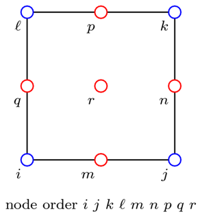
Nine-node quadrilateral elements are used to model the soil using the 9_4_QUadUP element. The connectivity for this type of element is depicted in Fig. 2. The input file automatically generates the elements based on the number of vertical elements specified in the mesh geometry section.
The self-weight of the soil is considered as a body force acting on each element. The body force is set as the saturated unit weight of the soil in each layer, which is determined from the respective saturated mass density input value.
Gravity Loading and Analysis
The gravity analysis in this example is conducted as a transient analysis with very large time steps, thus simulating a static analysis while avoiding the conflicts which may occur when mixing static and transient analyses. The self-weight of the soil elements provides the loads, therefore, no loading object is required. Gravity is applied for ten steps with entirely elastic constitutive behavior. This allows the material objects to update various parameters to account for confining pressure. Once these steps have converged, the material objects are updated using the updateMaterialStage command to consider elastoplastic behavior, and the gravity analysis is repeated for 40 steps.
Recorders
The recorders are defined after the gravity analysis so the recorded information only includes the post-gravity results. The recorders defined for this example document the following items:
- the nodal displacements in the displacement DOF
- the nodal velocities in the pore pressures DOF (records pore pressure data)
- the stress and strain response at the third Gauss point in each element
Consolidation Loading and Analysis
The consolidation loading comes from an surcharge load applied to the center node a the upper boundary of the soil layer (see Fig. 1). This load has a negative sign, and is applied in the vertical DOF, indicating that it is applied in the downward direction. The surcharge load is implemented using a constant timeseries and a plain pattern.
The consolidation analysis is also conducted as a transient analysis, and is analyzed for 400 steps with a time step of 0.25. The analysis is conducted using the Newmark integrator using the same gamma and beta coefficients defined in the gravity analysis.
Representative Results
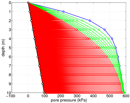
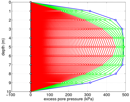
Several plots displaying results obtained from running this example analysis are provided for use as a means of verification and to demonstrate the information which can be gained from this 1D consolidation analysis. The distributions of excess pore pressure in the soil layer are shown Figs. 3 and 4 for the single and double drainage conditions, respectively. These figures show the initial distribution in blue. As time increases, the distributions transition from green to red. The final recorded time step is shown in black. As shown, the excess pore pressures in both cases approach zero with increasing time. More time steps would need to be considered to fully reach zero excess pore pressure for the single drainage condition. These figures were generated using the Matlab script plotPorePressure.m available for download in the compressed file at the top of this article.
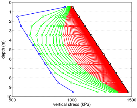
The distribution of vertical stress in the soil layer is shown in Fig. 5 for the case of double drainage. The same color scheme is used to indicate the passage of time. With increasing time and decreasing excess pore pressure, the vertical stress distribution approaches a linear variation dependent upon the soil unit weight. This figure was generated using the Matlab script plotStress.m available for download in the compressed file at the top of this article.
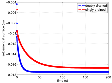
Fig. 6 shows the evolution of the settlement at the ground surface for the single and double drainage conditions. As would be expected, the settlement occurs more rapidly for the double drainage case. These figures were generated by plotting the recorded vertical displacements of the upper right node of the soil column at each time step.
