ElastomericX
This command is used to construct an ElastomericX bearing element object in three-dimension. The 3D continuum geometry of an elastomeric bearing is modeled as a 2-node, 12 DOF discrete element. This elements extends the formulation of Elastomeric_Bearing_(Plasticity)_Element (or Elastomeric_Bearing_(Bouc-Wen)_Element) elements, however, instead of an user providing material models as input arguments, it only takes geometric and material properties of an elastomeric bearing as arguments. The material models in six direction are formulated within the element from input arguments. In addition to the behavior captured by existing bearing elements, this element can capture the following:
- Coupled bidirectional motion in horizontal directions
- Coupling of vertical and horizontal motion
- Cavitation and post-cavitation behavior in tension
- Strength degradation in cyclic tensile loading due to cavitation
- Variation in critical buckling load capacity due to lateral displacement
For the full capabilities of this elements, users are referred to: EESD Article
The syntax of command to use this element in a 3D problem:
| element ElastomericX $eleTag $Nd1 $Nd2 $qRubber $uh $Gr $Kbulk $D1 $D2 $ts $tr $n <<$x1 $x2 $x3> $y1 $y2 $y3> <$kc> <$PhiM> <$ac> <$sDratio> <$m> <$cd> <$tc> |
| $eleTag | unique element object tag |
| $Nd1 $Nd2 | end nodes |
| $qRubber | yield strength |
| $uh | yield deformation |
| $Gr | shear modulus of elastomeric bearing |
| $Kbulk | bulk modulus of rubber |
| $D1 | internal diameter |
| $ts | single steel shim layer thickness |
| $tr | single rubber layer thickness |
| $n | number of rubber layers |
| $x1 $x2 $x3 | vector components in global coordinates defining local x-axis (optional) |
| $y1 $y2 $y3 | vector components in global coordinates defining local y-axis (optional) |
| $kc | cavitation parameter (optional, default = 10.0) |
| $PhiM | damage parameter (optional, default = 0.5) |
| $ac | strength reduction parameter (optional, default = 1.0) |
| $sDratio | shear distance from iNode as a fraction of the element length (optional, default = 0.5) |
| $m | element mass (optional, default = 0.0) |
| $cd | viscous damping parameter (optional, default = 0.0) |
| $tc | cover thickness (optional, default = 0.0) |
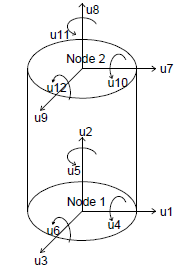
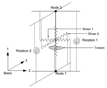
The physical model of an elastomeric bearing is considered as a two-node, twelve degrees-of-freedom discrete element. The two nodes are connected by six springs that represent the mechanical behavior in the six basic directions of a bearing. The degrees of freedom and discrete spring representation of an elastomeric bearing is shown in the below figures.
The general form of element force vector, <math>{{f}_{b}}</math>, and element stiffness matrix,<math>{{K}_{b}}</math> , for element representation considered above is given by equation below:
<math>{{f}_{b}}=\left[ \begin{matrix}
  Axial  \\
  Shear1  \\
  Shear2  \\
  Torsion  \\
  Rotation1  \\
  Rotation2  \\
\end{matrix} \right];\ \ \ \ \ \ {{K}_{b}}=\left[ \begin{matrix}
  Axial & 0 & 0 & 0 & 0 & 0  \\
  0 & Shear1 & Shear12 & 0 & 0 & 0  \\
  0 & Shear21 & Shear2 & 0 & 0 & 0  \\
  0 & 0 & 0 & Torsion & 0 & 0  \\
  0 & 0 & 0 & 0 & Rotation1 & 0  \\
  0 & 0 & 0 & 0 & 0 & Rotation2  \\
\end{matrix} \right]</math>
The coupling of the two shear springs is considered directly by using a coupled bidirectional model. All other springs are uncoupled. The coupling of vertical and horizontal directions are considered indirectly by using expressions for mechanical properties in one direction that are dependent on the response parameters in the other direction. Linear uncoupled springs are considered in the torsion and the two rotational springs as they are not expected to significantly affect the response of an elastomeric bearing. The off-diagonal terms due to coupling between axial and shear, and axial and rotation, are not considered in the two-spring model (Koh and Kelly, 1987) used here. An exact model would have non-zero values of these off-diagonal terms. A discussion on the formulation of the two-spring model and the exact model is presented in Ryan et al.(1991). The subscript refers to the element’s basic coordinate system. When the model is implemented in software programs, response quantities are transformed between the basic, local and global coordinates to perform computations.
The discrete spring model presented here has the advantages of easy implementation and being computationally efficient. The structural analysis software programs that allow user to add functionalities through user created elements (e.g., OpenSees and ABAQUS), provide a framework for such implementation. The mechanical properties of the six springs (also referred to as material models in OpenSees) are defined using analytical solutions available from the analysis of elastomeric bearings. These material models are discussed in the following sections. The expression for mechanical properties, including stiffness and buckling load capacity, are derived using explicit consideration for geometric nonlinearity due to large displacement effects. The P-Delta effect, which is an approximate method to account for geometric nonlinearity in structural analysis problems, is therefore not considered.
An example use of this element can be found here: File:DA.tcl
In this file a gravity load and a lateral offset is applied to the bearing. Then results are compared to the values that I had obtained my machine by displaying "Success" or "Failure"
References
- Kumar, M., Whittaker, A., and Constantinou, M. (2014). "An advanced numerical model of elastomeric seismic isolation bearings." Earthquake Engineering & Structural Dynamics, Published online, DOI: 10.1002/eqe.2431. Link

