Laterally-Loaded Pile Foundation: Difference between revisions
No edit summary |
No edit summary |
||
| Line 160: | Line 160: | ||
9. Vijayvergiya, V.N. (1977). “Load-movement characteristics of piles.” Proc., Ports 77 Conf., ASCE, New York. | 9. Vijayvergiya, V.N. (1977). “Load-movement characteristics of piles.” Proc., Ports 77 Conf., ASCE, New York. | ||
[[ | [[Examples| Return to OpenSees Examples Page]] | ||
Latest revision as of 18:38, 24 March 2011
Example prepared by: Christopher McGann and Pedro Arduino, University of Washington
Return to OpenSees Examples Page
This article describes the OpenSees implementation of a simple laterally-loaded pile example. The problem is modeled as a beam on a nonlinear Winkler foundation (BNWF), utilizing displacement-based beam elements for the pile and nonlinear spring elements which represent the vertical and lateral response of the surrounding soil. This example considers a static analysis only.
Provided with this article are the files needed to execute this analysis in OpenSees;
- the main input file, staticBNWFpile.tcl
- three procedures to define the soil constitutive behavior, get_pyParam.tcl, get_tzParam.tcl, and get_qzParam.tcl
- a file to define the pile section behavior, elasticPileSection.tcl
Download them all in a compressed file: staticBNWFanalysis.zip
To run this example, the user must download each of the above files and place them in a single directory. Once this has been done, the user can then type "source staticBNWFpile.tcl" into the interpreter of the OpenSees.exe application to run the analysis. Representative results are presented in this article to verify the correct implementation of this example. Additionally, the pile response obtained from this analysis is compared to a similar analysis conducted using the commercial program LPile (http://www.ensoftinc.com) to provide verification the results of the OpenSees analysis.
Model Description
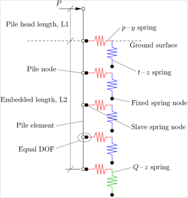
The BNWF model simulates the laterally-loaded pile problem using displacement-based beam elements to represent the pile and a series of nonlinear springs to represent the soil. The soil springs are generated using zero-length elements assigned separate uniaxial material objects in the lateral and vertical directions. An idealized schematic of the laterally-loaded pile model is provided in Fig. 1.
The pile axis is oriented in the z-coordinate direction, and all of the nodes are initially located on the z-axis (x- and y- coordinates are zero). Node numbering for each set of nodes begins at the bottom of the pile. The model is created with three separate sets of nodes:
- fixed spring nodes (numbers 1-85 in example)
- slave spring nodes (numbers 101-185 in example)
- pile nodes (numbers 201-285 in example)
Geometry and Mesh
The geometry is rather simple in this example. There is only a single layer of cohesionless soil, and the groundwater table is assumed to be well below the tip of the pile. The pile geometry controls the meshing of the problem. The user can specify the length of the pile head (above the ground surface), L1, and the embedded pile length (below the ground surface), L2. The default values in staticBNWFpile.tcl are L1 = 1 m, and L2 = 20 m. The pile is also assigned a diameter of 1 m. This value is used in the soil constitutive modeling.
The mesh is defined by the number of elements specified in the pile. The default value in this example is 84 elements (85 nodes). For the default pile geometry, this results in 80 elements over the embedded length and 4 elements above the ground surface. Note: The input file is only set up to handle up to 100 nodes. Modifications would need to be made to the node numbering scheme to accommodate a larger number of nodes.
Spring Nodes
The spring nodes are created with three dimensions and three translational degrees-of-freedom. The input file is set up to automatically generate the necessary spring nodes and elements based upon the input geometry (pile head length, $L1, embedded length, $L2, and number of pile elements, $nElePile). Spring nodes are only created over the embedded length of pile.
Since zero-length elements are used for the springs, the two sets of nodes share the same set of locations. One set of spring nodes, the fixed-nodes, are initially fixed in all three degrees-of-freedom. The other set of nodes, the slave nodes, are initially fixed in only two degrees-of-freedom, and are later given equal degrees-of-freedom with the pile nodes.
Spring Constitutive Behavior
The constitutive behavior of the springs is defined such that the springs oriented in the lateral direction represent p-y springs, and the vertically-oriented springs represent t-z and Q-z springs for the pile shaft and tip, respectively. Three procedures are used to properly define the p-y/t-z/Q-z behavior with depth, get_pyParam.tcl, get_tzParam.tcl, and get_qzParam.tcl
Several input soil properties are necessary to define these springs:
- soil unit weight, $gamma
- soil internal friction angle, $phi
- soil shear modulus, $Gsoil
The default values are set at $gamma = 17 kN/m^3, $phi = 36 degrees, and $Gsoil = 150000 kPa.
The procedure get_pyParam.tcl, which defines the p-y springs, has several options which must be selected.
- The first switch, $puSwitch, specifies the variation in ultimate lateral resistance with depth. The default, $puSwitch = 1, uses the recommendations of the American Petroleum Institute (API) (1993). The alternative method is that of Brinch Hansen (1961).
- The second switch, $kSwitch, specifies the variation in initial stiffness with depth. The default, $kSwitch = 1, specifies a linear variation of initial stiffness with depth (API 1993). The alternative uses a modified version of the API stiffness which varies parabolically with depth after Boulanger et al. (2003).
- The presence of groundwater can be accounted for in the initial stiffness using the third switch, $gwtSwitch. Default, $gwtSwitch = 1, is for no groundwater.
The other procedures, get_tzParam.tcl and get_qzParam.tcl, have no input options in this example. The t-z springs have behavior defined using the work of Mosher (1984) and Kulhawy (1991). The Q-z behavior is based on the work of Meyerhof (1976), Vijayvergiya (1977), and Kulhawy and Mayne (1990).
The p-y spring constitutive behavior is obtained using the PySimple1 uniaxial material object. The t-z and Q-z springs are defined using the TzSimple1 and QzSimple1 uniaxial materials, respectively. The main input file is set up to automatically generate the required spring material objects based upon the input geometry and soil properties.
Spring Elements
Zero-length elements are used for the soil springs using the element zeroLength. These elements connect the fixed and slave spring nodes. The the PySimple1 material objects are incorporated in the x-direction (direction of loading), while the TzSimple1, and at the pile tip, the QzSimple1, material objects are incorporated in the z-direction (vertical direction).
Pile Nodes
The pile nodes are created with three dimensions and six degrees-of-freedom (3 translational, 3 rotational). The input file is set up to automatically generate the necessary pile nodes and elements based upon the input geometry. A linear coordinate-transformation object is specified for the orientation of the pile in this example. With the exemption of the uppermost pile head node, the pile nodes are fixed against translation in the y-direction and rotations about the x- and z- axes. The pile head node, where the load is applied, is separated to allow the user to specify a free-head (no rotational fixity) or fixed-head (full rotational fixity) condition at the loading point.
The pile nodes over the embedded length of the pile are use linked with the slave spring nodes using the equalDOF command. The pile nodes are the master nodes in this example. These two sets of nodes share equal degrees-of-freedom in the x- and z- translational directions only.
Pile Constitutive Behavior and Elements
In this example, the pile is given elastic behavior for simplicity. Instead of using the elasticBeamColumn element, this is done using an elastic section object in conjunction with the displacement-based beam element, dispBeamColumn. This was done to facilitate future incorporation of elastoplastic pile section behavior using fiber section models by the user.
The properties of the elastic section for this example are defined in the file, elasticPileSection.tcl. The pile is defined with appropriately computed values for the cross-sectional area and the moments of inertia for its 1 m diameter, and is assigned a modulus of elasticity, E = 25000000, and shear modulus, G = 9615385.
Recorders
Several recorders are defined for this model.
- The displacements at the pile nodes in all three translational dof are recorded for use in extracting the displaced shape of the pile.
- The reaction forces in the p-y springs are recorded for use in visualizing the lateral soil response.
- The element forces in the pile elements are recorded in order to obtain shear and moment diagrams for the pile.
The recorders are set up to only record values at 0.5 second increments of pseudo-time during the analysis to facilitate the use of smaller load steps. This is done with the variable $timeStep.
A display recorder is included in the input file to allow the user to visualize the deformation of the pile in "real time" during the analysis. The parameters are set up for the orientation of the pile in this example.
Loading
This example considers a 3500 kN load applied in the positive x-direction at the head of the pile (uppermost pile node). This is accomplished in the model using a plain pattern with optional time-series parameters. The load increases linearly from 0 kN to 3500 kN over a 10 second increment of pseudo-time (between 10 and 20 seconds) and is then held constant after the loading period. Setting up the loading object in this manner allows for more control over the analysis.
Analysis
The analysis is conducted using the load-controlled integrator with a loading step of 0.05. This value is selected based on the 10 second interval specified in the loading object. 200 steps with a loading step of 0.05 will put the last step exactly at 10 seconds of pseudo-time. 201 steps are used in this example to make sure that the last recorded step is at the full loading magnitude. The variables $startT and $endT are used to print the cpu time needed to complete the analysis in the standard output or the OpenSees interpreter. The remaining analysis commands are well-documented in the OpenSees command manual.
Representative Results
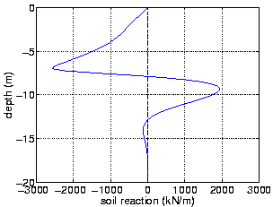
A user can verify their downloaded files by running the main input file, staticBNWFpile.tcl, in OpenSees and comparing the recorded results to some representative results included here. The simplest verification is to use the spring reaction forces recorded in the file reaction.out. A plot of the recorded spring reaction forces vs. depth in the final recorded pseudo-time step (20.05) should create something similar to that shown in Fig. 2. The response is negative from the ground surface to about 7.5 m deep, then transitions to positive until about 13 m deep, has a second smaller negative section, and then is nearly zero near the tip of the pile.
This verification plot can be made fairly simply using spreadsheet software. For those who prefer Matlab (http://www.mathworks.com/), the following lines will extract the desired information when pasted into an m-file.
% create depth vector
depth = linspace(-20,1,85);
% load data
react = load('reaction.out');
% remove pseudo-time information
react(:,1) = [];
% create plotting variable (divide by tributary area of pile to get force/length)
reactPlot = react(end,:)/0.25;
plot(reactPlot,depth)
The shear and moment diagram plots in the following section can also be used for verification purposes.
Comparison of OpenSees Results with LPile
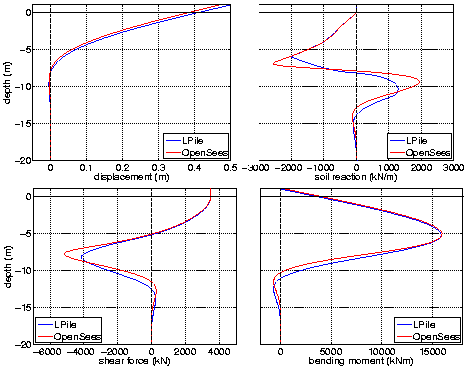
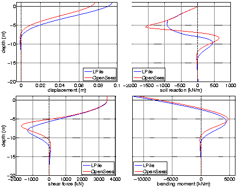
The commercial pile analysis program LPile (http://www.ensoftinc.com) is used to verify the results obtained using the OpenSees laterally-loaded pile model. The LPile analysis used the same geometric and constitutive parameters defined in the OpenSees analysis, and two cases were considered:
- A free-head case where there is no rotational fixity about the y-axis at the pile head
- A fixed-head case where full rotational fixity is enforced at the pile head.
The two analysis methods are compared via the recorded pile and soil responses. Figs. 3 and 4 present these comparisons for the free-head and fixed-head cases, respectively. Shown in these figures are the shear and moment diagrams, displaced pile shapes, and the lateral soil response recorded from each analysis. As shown, the LPile and OpenSees results are fairly similar, especially for the free-head case.
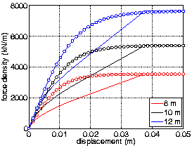
The main reason for the differences shown in Figs. 3 and 4 is that the p-y curves used in LPile are not the same as those used in the OpenSees analysis. The LPile curves are defined using the method of Reese et al. (1974), while the backbone of the p-y curves for the PySimple1 uniaxial material approximate the API (1993) recommendations. These two sets of curves are similar, and in fact have identical initial and ultimate responses, however, they vary in form over intermediate displacements.
This is shown in Fig. 5, which plots the actual p-y response obtained in the OpenSees simulation alongside the p-y curves used by LPile for several depths. As shown, the hyperbolic tangent curves recommended by the API do not match those used by LPile, especially for displacements between approximately 0.001 and 0.037 m. The force returned by the PySimple1 material object for displacements in this range will therefore be greater than corresponding forces used by LPile. This is confirmed by the soil response comparison plots in Figs. 3 and 4. Where the pile displacements are large, the LPile and OpenSees soil reactions are nearly identical, but as the displacements become smaller with increasing depth, the recorded soil reactions begin to differ. This difference in lateral soil response is the main reason behind the small variability observed in the recorded shear and moment diagrams and displaced shapes.
Overall, the agreement between the OpenSees and LPile analyses verifies that the BNWF model implemented in OpenSees is capable of returning sensible results for laterally-loaded pile simulations. There are differences between the results, however, these are relatively minor. The OpenSees simulation predicts maximum pile shear, moment, and deflection demands which are similar to those obtained from LPile, and the discrepancies are attributable to known differences between the two analysis methods.
References
1. American Petroleum Institute (API) (1987). Recommended Practice for Planning, Designing and Constructing Fixed Offshore Platforms. API Recommended Practice 2A(RP-2A), Washington D.C, 17th edition.
2. Brinch Hansen, J. (1961). “The ultimate resistance of rigid piles against transversal forces.” Bulletin No. 12, Geoteknisk Institute, Copenhagen, 59.
3. Boulanger, R. W., Kutter, B. L., Brandenberg, S. J., Singh, P., and Chang, D. (2003). Pile Foundations in liquefied and laterally spreading ground during earthquakes: Centrifuge experiments and analyses. Center for Geotechnical Modeling, University of California at Davis, Davis, CA. Rep. UCD/CGM-03/01.
4. Kulhawy, F.H. (1991). "Drilled shaft foundations." Foundation engineering handbook, 2nd Ed., Chap 14, H.-Y. Fang ed., Van Nostrand Reinhold, New York.
5. Kulhawy, F.H. and Mayne, P.W. (1990). Manual on Estimating Soil Properties for Foundation Design. Electrical Power Research Institute. EPRI EL-6800, Project 1493-6 Final Report.
6. Meyerhof G.G. (1976). "Bearing capacity and settlement of pile foundations." J. Geotech. Eng. Div., ASCE, 102(3), 195-228.
7. Mosher, R.L. (1984). “Load transfer criteria for numerical analysis of axial loaded piles in sand.” U.S. Army Engineering and Waterways Experimental Station, Automatic Data Processing Center, Vicksburg, Miss.
8. Reese, L.C. and Van Impe, W.F. (2001), Single Piles and Pile Groups Under Lateral Loading. A.A. Balkema, Rotterdam, Netherlands.
9. Vijayvergiya, V.N. (1977). “Load-movement characteristics of piles.” Proc., Ports 77 Conf., ASCE, New York.